Everything starts with simple steps, so does machine learning. This post will talk about regression supervise learning. If you’re not familiar with some term, I suggest you to enroll machine learning class from coursera. The idea is to give prediction regarding current data/training set available, represented in form of linear equation.
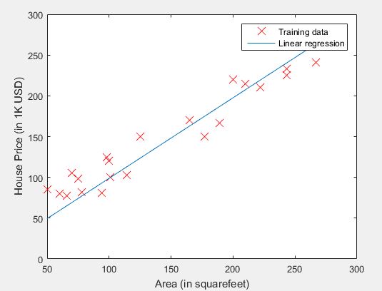
For example, let’s see figure below:

Image above describe relation between total area of the house (in squarefeet) and house price (in 1K USD). Let’s say I want to sell my house (112 squarefeet). By using this data, I want to predict how much should I sell my house. The idea is to create model using linear equation that is close enough to form function of above image. For this writing purpose, I will simplify the form of equation to become a vectorized form so that we can easily adapt it into matlab.
First step is to create hypothesis function, defined by linear equation below:

The vectorized form for above equation is:

where 


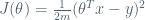
Next idea is to minimize some function that has relation between our hypothesis function, and the actual house price. This is a building block of supervised learning algorithm, referred as cost function J, defined as follows:

The vectorized form is:
where 


The vectorized form is:

where 
The implementation in Matlab is roughly like this
function J = computeCost(X, y, theta)
    m = length(y); % number of training examples

    %calculate J function by using vectorized
    J = sum((transpose(theta) * X - y).^2)/(2*m);
end

function [theta, J_history] = gradientDescent(X, y, theta, alpha, iters)
	m = length(y); % number of training examples
	J_history = zeros(num_iters, 1);

	for iter = 1:iters %for converged function purposes
		J_history(iter) = computeCost(X, y, theta);

		h = X * theta; %hypothesis function
		diff = h - y; %delta between hypothesis function and actual price

		%compute the new theta value by executing the derivation equation
		theta_change = (diff * transpose(X) .* alpha) /m;
		theta = theta - transpose(theta_change);

		%make sure cost function J is always decreasing
		fprintf('%f %f %f \n', J_history(iter), theta(1), theta(2));

	end
end
In this calculation, I use 
12085.976190 0.001446 0.240599
7001.842606 0.002555 0.422608
4092.378664 0.003408 0.560293
2427.398658 0.004068 0.664450
1474.591315 0.004581 0.743243
929.334352 0.004985 0.802847
617.303572 0.005304 0.847937
438.739612 0.005560 0.882047
...
199.313357 0.094885 0.987497
199.313004 0.094944 0.987496
199.312650 0.095004 0.987496
Theta found by gradient descent: 0.095004 0.987496
For area 112, we predict a price of 110.694545
By above result, the hypothesis function is defined as follow:
The result of linear regression figure can be seen below:

Cheers!
